1. Intro to linear regression

Press the button 'Toggle code' below to toggle code on and off for entire this presentation.

from IPython.display import display
from IPython.display import HTML
import IPython.core.display as di # Example: di.display_html('<h3>%s:</h3>' % str, raw=True)

# This line will hide code by default when the notebook is exported as HTML
di.display_html('<script>jQuery(function() {if (jQuery("body.notebook_app").length == 0) { jQuery(".input_area").toggle(); jQuery(".prompt").toggle();}});</script>', raw=True)

# This line will add a button to toggle visibility of code blocks, for use with the HTML export version
di.display_html('''<button onclick="jQuery('.input_area').toggle(); jQuery('.prompt').toggle();">Toggle code</button>''', raw=True)

Toggle code

1. Intro to linear regression

With linear regression we aim to fit a line (or hyperplane in higher dimensions) to a scattering of data. In this Section we describe the fundamental concepts underlying this procedure.

1.1 Notation and modeling

Data for regression problems comes in the form of a set of $P$ input/output observation pairs

\begin{equation} \left(\mathbf{x}_{1},y_{1}\right),\,\left(\mathbf{x}_{2},y_{2}\right),\,...,\,\left(\mathbf{x}_{P},y_{P}\right) \end{equation}

or $\left\{ \left(\mathbf{x}_{p},y_{p}\right)\right\} _{p=1}^{P}$ for short, where $\mathbf{x}_{p}$ and $y_{p}$ denote the $p^{\textrm{th}}$ input and output respectively.

In general each input $\mathbf{x}_{p}$ may be a column vector of length $N$

\begin{equation} \mathbf{x}_{p}=\left[\begin{array}{c} x_{1,p}\\ x_{2,p}\\ \vdots\\ x_{N,p} \end{array}\right] \end{equation}

in which case the linear regression problem is analogously one of fitting a hyperplane to a scatter of points in $N+1$ dimensional space.

In the case of scalar input the fitting of a line to the data requires we determine a vertical intercept $w_0$ and slope $w_1$ so that the following approximate linear relationship holds between the input/output data

\begin{equation} w_{0}+x_{p}w_{1}\approx y_{p},\quad p=1,...,P. \end{equation}

More generally, when dealing with $N$ dimensional input we have a bias and $N$ associated slope weights to tune properly in order to fit a hyperplane, with the analogous linear relationship written as

\begin{equation} w_{0}+ x_{1,p}w_{1} + x_{2,p}w_{2} + \cdots + x_{N,p}w_{N} \approx y_{p} ,\quad p=1,...,P. \end{equation}

For any $N$ we can write the above more compactly by denoting

\begin{equation} \mathbf{w}=\left[\begin{array}{c} w_{1}\\ w_{2}\\ \vdots\\ w_{N} \end{array}\right] \end{equation}

as

\begin{equation} w_0+\mathbf{x}_{p}^T\mathbf{w} \approx y_{p} ,\quad p=1,...,P. \end{equation}

1.2 The Least Squares cost function

• To find the parameters of the hyperplane which best fits a regression dataset we form a Least Squares cost function.

• For a given set of parameters $\mathbf{w}$ this cost function computes the total squared error between the associated hyperplane and the data.

We want to find a weight vector $\mathbf{w}$ and the bias $w_0$ so that each of following $P$ approximate equalities holds as well as possible.

\begin{equation} w_0+\mathbf{x}_{p}^T\mathbf{w} \approx y_{p} \end{equation}

Another way of stating the above is to say that the error between $w_0+\mathbf{x}_{p}^{T}\mathbf{w}$ and $y_{p}$ is small.

\begin{equation} \left(w_0+\mathbf{x}_{p}^{T}\mathbf{w} - y_{p}^{\,}\right)^2 \end{equation}

\begin{equation} \,g\left(w_0,\mathbf{w}\right)=\sum_{p=1}^{P}\left(w_0+\mathbf{x}_{p}^{T}\mathbf{w}-y_{p}^{\,}\right)^{2} \end{equation}

• We want parameters $w_0$ and $\mathbf{w}$ that provide a small value for $g\left(w_0,\mathbf{w}\right)$

• In other words, we want to determine a value for the pair $w_0$ and $\mathbf{w}$ that minimizes $g\left(w_0,\mathbf{w}\right)$,

\begin{equation} \underset{w_0,\,\mathbf{w}}{\mbox{minimize}}\,\,\underset{p=1}{\overset{P}{\sum}}\left(w_0+\mathbf{x}_{p}^{T}\mathbf{w}-y_{p}^{\,}\right)^{2} \end{equation}

Here is what we will see

# animate descent process
demo2.animate_it_3d(w_hist,view = [10,-40],viewmax = 1.3)

• how can we do this?

2. Intro to gradient descent

2.1 The gradient descent direction

# what function should we play with?  Defined in the next line.
g = lambda w: 0.4*w**2 + 1.5

# run the visualizer for our chosen input function
callib.derivative_ascent_visualizer.animate_visualize2d(g=g,num_frames = 150,plot_descent = True)

• The gradient: a partial derivative in each input coordinate direction

• e.g., if $N = 2$

\begin{equation} \nabla g(w_1,w_2) = \begin{bmatrix} \ \frac{\partial}{\partial w_1}g(w_1,w_2) \\ \frac{\partial}{\partial w_2}g(w_1,w_2) \end{bmatrix} \end{equation}

# define function, and points at which to take derivative
func = lambda w:  (w[0])**2 + (w[1])**2 + 6
pt1 = [-1,1];

# animate 2d slope visualizer
view = [33,30]
callib.derivative_ascent_visualizer.visualize3d(func=func,view = view,pt1 = pt1,plot_descent = True)

• The negative gradient provides descent direction - always - unless at a stationary point

2.2 Intuition for gradient descent

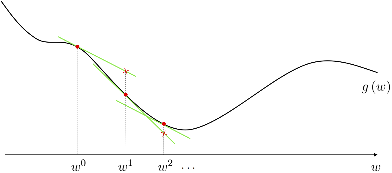
• Its like trying to find your way downhill in the complete dark

• To the keynote cartoon!

2.3 Basic gradient descent algorithm

These update steps are written mathematically - when $N = 1$ - as

\begin{equation} w^{\,k} = w^{\,k-1} - \alpha \frac{\mathrm{d}}{\mathrm{d}w}g\left(w^{\,k-1}\right) \end{equation}

And when $N \geq1$ more generally as

\begin{equation} \mathbf{w}^{\,k} = \mathbf{w}^{\,k-1} - \alpha \nabla g(\mathbf{w}^{\,k-1}) \end{equation}

• Here $\alpha$ is called the steplength parameter or learning rate

The length of each descent step

• We will see how to choose the steplength parameter $\alpha$ soon

• Note: here the length of each step is precisely $\alpha\left\Vert \nabla g\left(\mathbf{w}^{\,k-1}\right) \right\Vert_2$, not just the steplength parameter itself.

A demo

Minimize the function

\begin{equation} g(w) = \frac{1}{50}\left(w^4 + w^2 + 10w\right) \end{equation}

• has very difficult to compute (by hand) global minimum

\begin{equation} w = \frac{\sqrt[\leftroot{-2}\uproot{2}3]{\sqrt[\leftroot{-2}\uproot{2}3]{2031} - 45}}{6^{\frac{2}{3}}} - \frac{1}{\sqrt[\leftroot{-2}\uproot{2}3]6\left(\sqrt{2031}-45\right)} \end{equation}

# what function should we play with?  Defined in the next line.
g = lambda w: 1/float(50)*(w**4 + w**2 + 10*w)   # try other functions too!  Like g = lambda w: np.cos(2*w) , g = lambda w: np.sin(5*w) + 0.1*w**2, g = lambda w: np.cos(5*w)*np.sin(w)

# run the visualizer for our chosen input function, initial point, and step length alpha
demo = optlib.gradient_descent_demos.visualizer();

demo.animate_2d(g=g, w_init = 2.5,steplength = 0.5,max_its = 45,version = 'unnormalized')

Steplength selection in general

# what function should we play with?  Defined in the next line., nice setting here is g = cos(2*w), w_init = 0.4, alpha_range = np.linspace(2*10**-4,1,200)
g = lambda w: w**2

# create an instance of the visualizer with this function
demo = optlib.grad_descent_steplength_adjuster_2d.visualizer()

# run the visualizer for our chosen input function, initial point, and step length alpha
w_init = -2.5
steplength_range = np.linspace(10**-5,1.5,150)
max_its = 5
demo.animate_it(w_init = w_init, g = g, steplength_range = steplength_range,max_its = max_its,tracers = 'on',version = 'unnormalized')