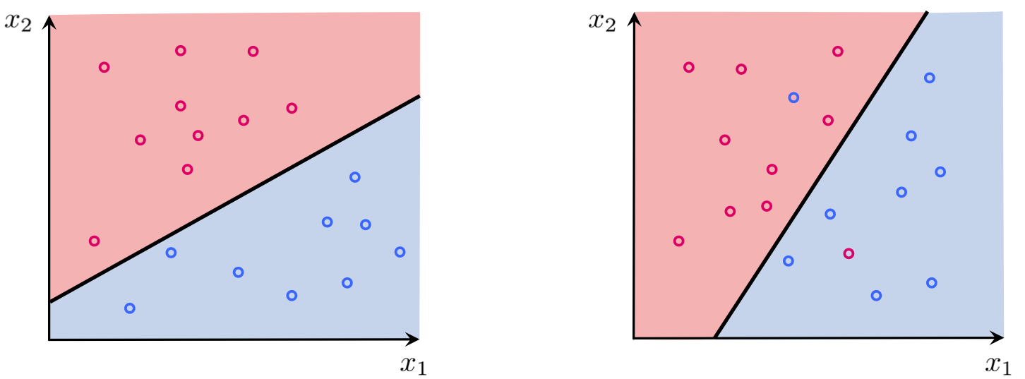
In this post we discuss the perceptron - a historically significant and useful way of thinking about linear classification.
Press the button 'Toggle code' below to toggle code on and off for entire this presentation.
from IPython.display import display
from IPython.display import HTML
import IPython.core.display as di # Example: di.display_html('<h3>%s:</h3>' % str, raw=True)

# This line will hide code by default when the notebook is exported as HTML
di.display_html('<script>jQuery(function() {if (jQuery("body.notebook_app").length == 0) { jQuery(".input_area").toggle(); jQuery(".prompt").toggle();}});</script>', raw=True)

# This line will add a button to toggle visibility of code blocks, for use with the HTML export version
di.display_html('''<button onclick="jQuery('.input_area').toggle(); jQuery('.prompt').toggle();">Toggle code</button>''', raw=True)
1. The perceptron
In this Section we derive the perceptron, which provides a foundational perceptron perspective on two-class classification. We will see - among other things - our first use of the rectified linear unit as well as the origin of phrase softmax in softmax cost function.
1.1 The perceptron cost function
With two-class classification we have a training set of $P$ points $\left\{ \left(\mathbf{x}_{p},y_{p}\right)\right\} _{p=1}^{P}$ where $y_p$'s take on just two label values from $\{-1, +1\}$.
As we saw with logistic regression the decision boundary was formally given as a hyperplane
\begin{equation} w_0+\mathbf{x}^{T}\mathbf{w}^{\,} = 0 \end{equation}When hyperplane parameters $w_0$ and $\mathbf{w}$ are chosen well we have (for most points)
\begin{equation} \begin{array}{cc} w_0+\mathbf{x}_{p}^{T}\mathbf{w}>0 & \,\,\,\,\text{if} \,\,\, y_{p}=+1\\ w_0+\mathbf{x}_{p}^{T}\mathbf{w}<0 & \,\,\,\,\text{if} \,\,\, y_{p}=-1 \end{array} \end{equation}

The two (ideal) conditions again:
\begin{equation} \begin{array}{cc} w_0+\mathbf{x}_{p}^{T}\mathbf{w}>0 & \,\,\,\,\text{if} \,\,\, y_{p}=+1\\ w_0+\mathbf{x}_{p}^{T}\mathbf{w}<0 & \,\,\,\,\text{if} \,\,\, y_{p}=-1 \end{array} \end{equation}We can combine them in a single equation (because $y_p \in \{-1,+1\}$)
\begin{equation} -y_{p}\left(w_0+\mathbf{x}_{p}^{T}\mathbf{w}\right)<0 \end{equation}written equivalently - using ReLU function - as
\begin{equation} \text{max}\left(0,\,-y_{p}\left(w_0+\mathbf{x}_{p}^{T}\mathbf{w}\right)\right)=0 \end{equation}Lets look at the expression $\text{max}\left(0,\,-y_{p}\left(w_0+\mathbf{x}_{p}^{T}\mathbf{w}\right)\right)$ more closely:
- It is always non-negative: it returns zero if $\mathbf{x}_{p}$ is classified correctly, and returns a positive value if classified incorrectly.
- It is convex: because it is the composition of ReLU (itself a convex function) and a linear function.
We sum up this expression over the entire dataset, giving the so-called perceptron or ReLU cost
\begin{equation} g\left(w_0,\mathbf{w}\right)=\underset{p=1}{\overset{P}{\sum}}\text{max}\left(0,\,-y_{p}\left(w_0+\mathbf{x}_{p}^{T}\mathbf{w}\right)\right) \end{equation}The ReLU cost
\begin{equation} g\left(w_0,\mathbf{w}\right)=\underset{p=1}{\overset{P}{\sum}}\text{max}\left(0,\,-y_{p}\left(w_0+\mathbf{x}_{p}^{T}\mathbf{w}\right)\right) \end{equation}- is convex: because each summand is convex!
- has only a single (discontinuous) derivative: because of the ReLU function. Therefore we can only use first order methods for its optimization.
- has a trivial and undesired solution at zero: when $w_0=0$ and $\mathbf{w} = \mathbf{0}$, we have $g\left(0,\mathbf{0}\right) = 0$.
Example 1: Using gradient descent to minimize the ReLU cost
We test out the perceptron on the 3-d dataset used in the previous (logistic regression) example
The perceptron / relu cost function - a Python implementation
# the relu cost function
def relu(w):
    cost = 0
    for p in range(0,len(y)):
        x_p = x[p]
        y_p = y[p]
        a_p = w[0] + sum([a*b for a,b in zip(w[1:],x_p)])
        cost += np.maximum(0,-y_p*a_p)
    return cost
# declare an instance of our current our optimizers
opt = superlearn.optimimzers.MyOptimizers()

# run desired algo with initial point, max number of iterations, etc.,
w_hist = opt.gradient_descent(g = relu,w = np.random.randn(np.shape(x)[1]+1,1),max_its = 50,alpha = 10**-2,steplength_rule = 'diminishing')

# create instance of 3d demos
demo5 = superlearn.classification_3d_demos.Visualizer(data)

# draw the final results
demo5.static_fig(w_hist,view = [15,-140])
1.2 The smooth softmax approximation to the ReLU perceptron cost
The softmax function defined as
\begin{equation} \text{soft}\left(s_1,s_2,...,s_N\right) = \text{log}\left(e^{s_1} + e^{s_2} + \cdots + e^{s_N} \right) \end{equation}is a generic smooth approximation to the max function
\begin{equation} \text{soft}\left(s_1,s_2,...,s_N\right) \approx \text{max}\left(s_1,s_2,...,s_N\right) \end{equation}Why? Say, $s_j$ is the maximum and (much) larger than the rest. Then, $e^{s_{j}}$ dominates the sum and we have that
\begin{equation} \text{log}\left(e^{s_1} + e^{s_2} + \cdots + e^{s_N} \right) \approx \text{log}\left(e^{s_j} \right) = s_j \end{equation}Example 1: Softmax approximation to the ReLU
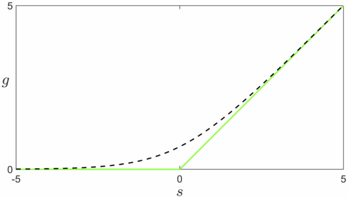
The ReLU function
\begin{equation} g\left(s\right)=\mbox{max}\left(0,\,s\right) \end{equation}and its smooth softmax approximation
\begin{equation} g\left(s\right)=\mbox{soft}\left(0,\,s\right)=\mbox{log}\left(1+e^{s}\right) \end{equation}

Recall the ReLU perceptron cost function
\begin{equation} g\left(w_0,\mathbf{w}\right)=\underset{p=1}{\overset{P}{\sum}}\text{max}\left(0,\,-y_{p}\left(w_0+\mathbf{x}_{p}^{T}\mathbf{w}\right)\right) \end{equation}We replace the $p^{th}$ summand with its softmax approximation
\begin{equation} \text{soft}\left(0,\,-y_{p}\left(w_0+\mathbf{x}_{p}^{T}\mathbf{w}\right)\right)= \text{log}\left(e^{0} + e^{-y_{p}\left(w_0+\mathbf{x}_{p}^{T}\mathbf{w}\right)}\right) = \text{log}\left(1 + e^{-y_{p}\left(w_0+\mathbf{x}_{p}^{T}\mathbf{w}\right)}\right) \end{equation}giving the smooth cost function
\begin{equation} g\left(w_0,\mathbf{w}\right)=\underset{p=1}{\overset{P}{\sum}}\text{log}\left(1 + e^{-y_{p}\left(w_0+\mathbf{x}_{p}^{T}\mathbf{w}\right)}\right) \end{equation}Where have you seen this cost before?
\begin{equation} g\left(w_0,\mathbf{w}\right)=\underset{p=1}{\overset{P}{\sum}}\text{log}\left(1 + e^{-y_{p}\left(w_0+\mathbf{x}_{p}^{T}\mathbf{w}\right)}\right) \end{equation}- This is the softmax cost previously derived from the logistic regression perspective on two-class classification.
- It is called softmax since it derives from the general softmax approximation to the max function.
- It is still convex (like the ReLU cost) but no trivial solution at zero!
1.3 Predictions, misclassifications, and accuracy with the perceptron cost
Predictions, misclassifications, the accuracy, etc., are all found in the same manner described for logistic regression.