Nonlinear supervised learning
Press the button 'Toggle code' below to toggle code on and off for entire this presentation.
from IPython.display import display
from IPython.display import HTML
import IPython.core.display as di # Example: di.display_html('<h3>%s:</h3>' % str, raw=True)

# This line will hide code by default when the notebook is eåxported as HTML
di.display_html('<script>jQuery(function() {if (jQuery("body.notebook_app").length == 0) { jQuery(".input_area").toggle(); jQuery(".prompt").toggle();}});</script>', raw=True)

# This line will add a button to toggle visibility of code blocks, for use with the HTML export version
di.display_html('''<button onclick="jQuery('.input_area').toggle(); jQuery('.prompt').toggle();">Toggle code</button>''', raw=True)
1.1 From linear to non-linear modeling
- Thus far we have covered the basics of linear modeling for regression and classification.
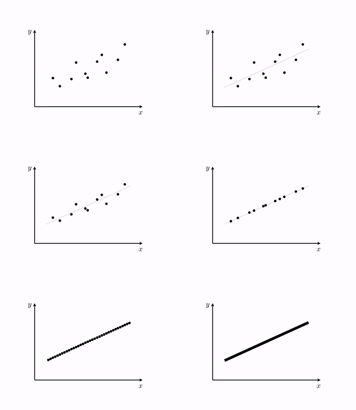
- With regression we started with a desire that a dataset could be represented linearly via the model $w_0 + \mathbf{x}_p^T\mathbf{w}_{\,}^{\,} \approx y_p$
- This desire led to the Least Squares cost function for linear regression, which minimized provokes our desire to hold as well as possible.
- So, in other words, ideally we want all our data to lie on some hyperplane $w_0^{\,} + \mathbf{x}_{\,}^T\mathbf{w}_{\,}^{\,} = y_{\,}^{\,}$ in the input/output space
- So our ideal dataset is a bunch of points - with no noise - from a hyperplane
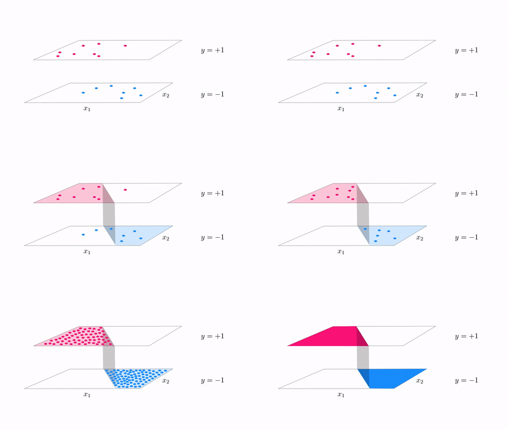
- With classification we started with a desire that a dataset could be represented linearly the step function with linear boundary
- A hyperplane in the input space $w_0 + \mathbf{x}_{\,}^T\mathbf{w}_{\,}^{\,} = 0$ where
- In other ideally we want data to lie perfectly on a step function $\text{sign}\left(w_0 + \mathbf{x}_{\,}^T\mathbf{w}_{\,}^{\,} \right) = y$
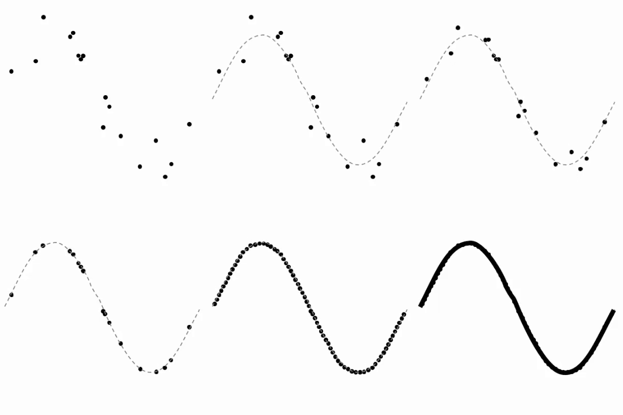
The generalization of this notion for regression
- for regression: our data lies perfectly on a nonlinear
hyperplanesurface
- instead of hyperplane $w_0^{\,} + \mathbf{x}_{\,}^T\mathbf{w}_{\,}^{\,} = y_{\,}^{\,}$ we have some general nonlinear function $f\left(\mathbf{x},\mathbf{w}\right) = y$
- as with linear regression we do not expect perfection!
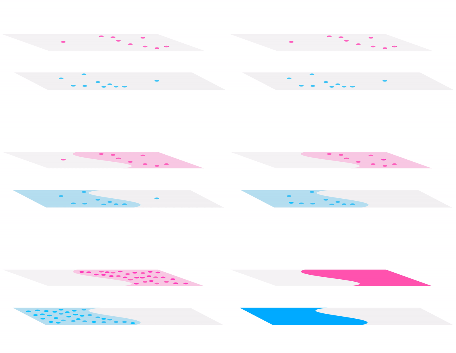
The generalization of this notion for classification
- for classification: our data lies perfectly on step function with
linearnonlinear boundary
- instead of separating hyperplane $w_0^{\,} + \mathbf{x}_{\,}^T\mathbf{w}_{\,}^{\,} = 0$ we have some general nonlinear seperator $f\left(\mathbf{x},\mathbf{w}\right) = 0$
- as with linear classification we do not expect perfection!
1.2 'Simple' examples of nonlinear regression and classification
- For some low-dimensional datasets we could visualize and reason out a proper nonlinear function / separator by eye
- In some classical cases from e.g., physics and economics one can reason out the form of a regressor via philisophical arguments
- (This is what differential equations and dynamical systems are all about)
- In general cannot rely on either our eyes or understanding in general to provide nonlinear form
- Most datasets too high dimensional to visualize, and mechanics lie beyond our comprehension
- So in general we need something more robust - this is where machine learning comes in!
- Tools like neural networks help automate the search for proper nonlinear regressors / boundaries (as do trees and kernels)
- First lets examine some 'easy' cases where we can make a good guess ourselves
- Some important principles, formulations, jargon, etc., from these simple cases carry over to neural networks, trees, kernels, etc.,
'Simple' nonlinear regression examples
Example 1. A sinusoidal dataset
# create instance of linear regression demo, used below and in the next examples
demo1 = nonlib.nonlinear_regression_visualizer.Visualizer(csvname = datapath + 'noisy_sin_sample.csv')
demo1.plot_data(xlabel = 'x',ylabel = 'y')
- Looks sinusoidal, i.e., like
could fit the data well if parameters are tuned
- This would give us a nonlinear regressor or predictor of the form
- How do we fit? As in the linear case we want the above to hold on our data lets square their differences, and minimize a Least Squares cost
- Summing over all $P$ datapoints gives the Least Squares cost function
- Minimize this by (normalized) gradient descent
- In Python implementation we break the cost into modular pieces
- the sine nonlinearity --> the prediction --> the cost function
# nonlinearity
def f(x_val,w):
    # create feature
    f_val = np.sin(w[2] + w[3]*x_val)
    return f_val

# prediction
def predict(x_val,w):
    # linear combo
    val = w[0] + w[1]*f(x_val,w)
    return val

# least squares
def least_squares(w):
    cost = 0
    for p in range(0,len(y)):
        x_p = x[p]
        y_p = y[p]
        cost +=(predict(x_p,w) - y_p)**2
    return cost
Now we can minimize the cost using gradient descent
We can then plot the resulting fit to the data
# static transform image
demo1.static_img(w_best,least_squares,predict)
- Some common jargon to familiarize yourself with: we have already seen (now all weights are tuned)
- In particular the nonlinear transformation of $x$ is called a feature transformation (we wrote this explicitly in code)
- We can write the predictor as
- We can write the predictor as
- In other words, the predictor is a linear combination of the feature transform $f(x)$
- Thus in the transformed feature space with input horizontal axis $f(x)$ and vertical axis $y$ our sinusoidal fit is linear
# static transform image
demo1.static_img(w_best,least_squares,predict,f1_x = [f(v,w_best) for v in x])
- This is true in general
A properly designed feature (or set of features) provides a good nonlinear fit in the original feature space and, simultaneously, a good linear fit in the transformed feature space.
Example 2. A population growth example
Next we examine a population growth dataset - of Yeast cells growing in a constrained enviroment (source).
Both input and output normalized
# create instance of linear regression demo, used below and in the next examples
demo2 = nonlib.nonlinear_regression_visualizer.Visualizer(csvname = datapath + 'yeast.csv')

# plot dataset
demo2.plot_data(xlabel = 'time', ylabel = 'yeast population')
- What does this look like?
- Certainly looks like a sigmoidal regressor would do the job well here
- Here $f(x) = \text{tanh}\left(w_2 + w_3x\right)$ is our feature transformation, and we minimize the Least Squares error
- Once weights tuned properly this provides linear fit in transformed feature space
# nonlinearity
def f(x,w):
    # shove through nonlinearity
    c = np.tanh( w[2] + w[3]*x)
    return c

# prediction
def predict(x,w):
    # linear combo
    val = w[0] + w[1]*f(x,w)
    return val

# least squares
def least_squares(w):
    cost = 0
    for p in range(0,len(y)):
        x_p = x[p]
        y_p = y[p]
        cost +=(predict(x_p,w) - y_p)**2
    return cost
- Center data and minimize via normalized gradient descent
# static transform image
demo2.static_img(w_best,least_squares,predict,f1_x = [f(v,w_best) for v in x])
- On the right - data in transformed feature space (note again all weights are now tuned)
Example 3. Galileo's ramp experiment
- In 1638 Galileo wants to understand how gravity acts on objects quantify the relationship between
- In particular: how does an object's distance from above ground affect the time it takes to hit the ground when dropped
- Sets up the following experiment

- Why didn't he just drop the ball and time how long it took to get $\frac{1}{4}$, $\frac{1}{2}$, etc., to the ground?
- Reliable clocks didn't exist yet! (he used a water clock.) Galielo's later study of pendulums led to first realiable clock
- He performed this experiment many times and averaged the results, got data like this (from a modern reenactment)
# create instance of linear regression demo, used below and in the next examples
demo3 = nonlib.nonlinear_regression_visualizer.Visualizer(csvname = datapath + 'galileo_ramp_data.csv')

# plot dataset
demo3.plot_data(xlabel = 'time (in seconds)',ylabel = 'portion of ramp traveled')
- Clearly a nonlinear relationship - Galileo intuitied a quadratic one
- In other words, that for some $w_0$, $w_1$, and $w_2$ that
- Here we have 2 feature transformations: the identity $f_1(x) = x$ and $f_2(x) = x^2$ so can write
- Recover weights by minimizing Least Squares error
# feature transformation
def f1(x):
    return x

def f2(x):
    return x**2

# prediction
def predict(x,w):
    # linear combo
    a = w[0] + w[1]*f1(x) + w[2]*f2(x)
    return a

# least squares
def least_squares(w):
    cost = 0
    for p in range(0,len(y)):
        x_p = x[p]
        y_p = y[p]
        cost +=(predict(x_p,w) - y_p)**2
    return cost
And we optimize using e.g., (unnormalized) gradient descent
# static transform image
f1_x = [f1(v) for v in x]; f2_x = [f2(v) for v in x]
demo3.static_img(w_best,least_squares,predict,f1_x=f1_x,f2_x=f2_x,view = [35,100])
- Here the linear fit is in one dimension higher than where we started!
- True more generally speaking: the more feature transforms we use the higher up we go!
'Simple' nonlinear classification examples
Example 4. A one dimensional example
- With linear regression we started with a desire that a dataset could be represented linearly via the model $w_0 + {w}_{1}^{\,}{x}_p \approx y_p$
- With logistic regression we started with a desire that a dataset could be represented by shoving line through sigmoid as in $\text{tanh}\left(w_0 + {w}_{1}^{\,}{x}_p\right) \approx y_p$
- Once tuned our decision boundary $w_0 + w_1x = 0$, our decision boundary
- Our predictor is then
- If $\text{predict}(x) > 0$ then $x$ assigned to $+1$ class, if $\text{predict}(x) < 0$ assigned to $-1$ class
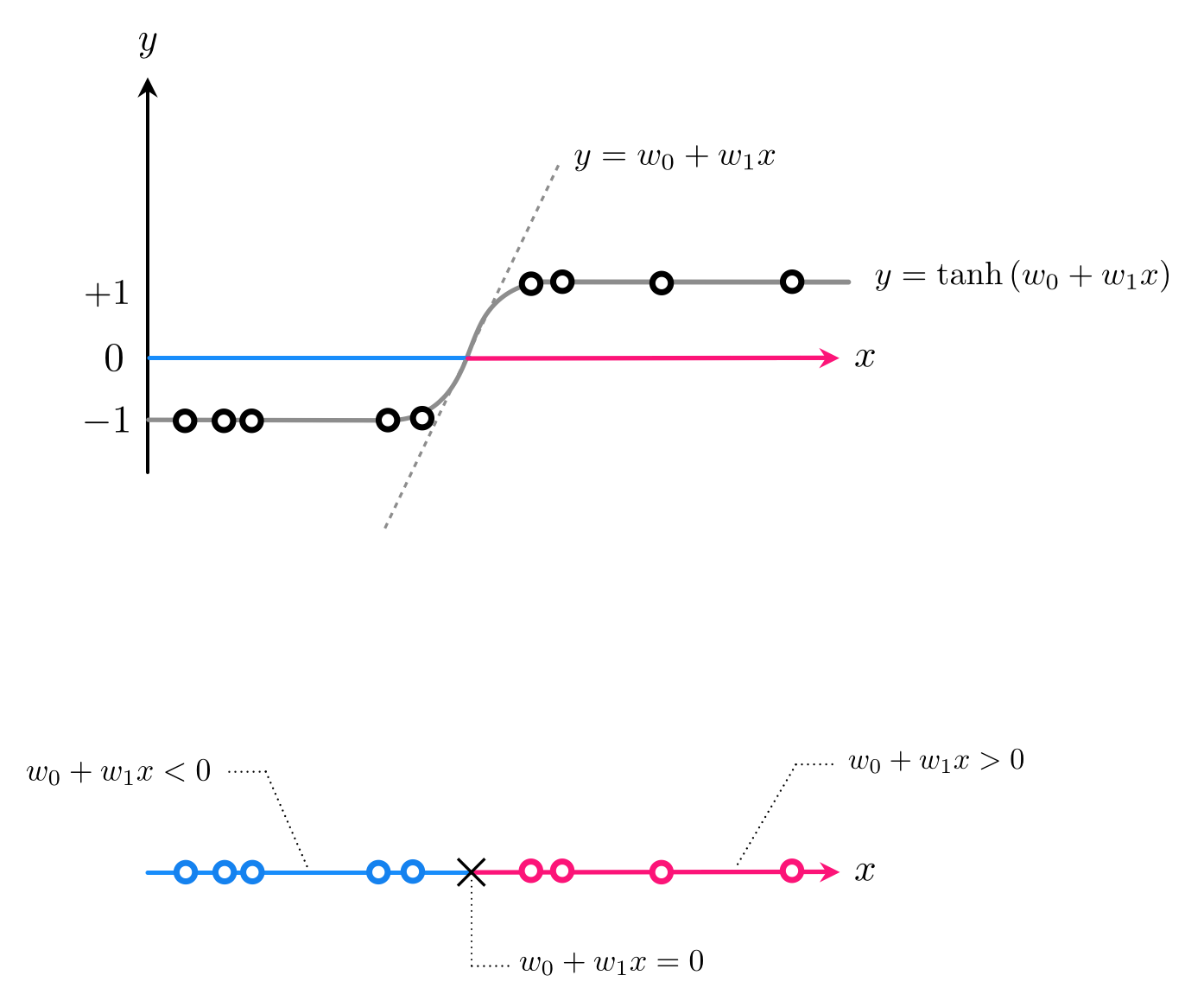
- Tune by minimizing e.g., softmax cost
- What about this dataset?
# create instance of linear regression demo, used below and in the next examples
demo4 = nonlib.nonlinear_classification_visualizer.Visualizer(csvname = datapath + 'signed_projectile.csv')

# plot dataset
demo4.plot_data()
- How about a quadratic decision boundary: $w_0 + w_1x^{\,} + w_2x^2 = 0$
- If we denote
then once tuned if $\text{predict}(x) > 0$ $x$ in class $+1$, if $\text{predict}(x)<0$ class $-1$
- Here we have two feature transformations (we will write explicitly in code)
- So we can write our predictor
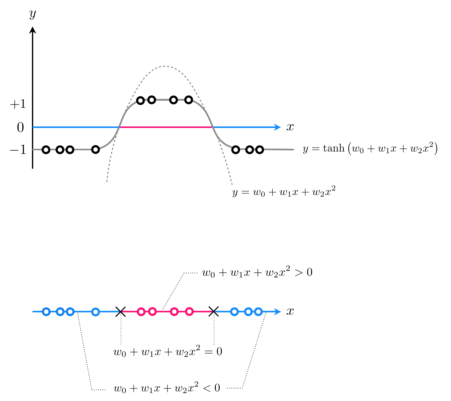
- Tune weights by minimizing e.g., the softmax cost: $\,g\left(w_0,w_1,w_2\right) = \sum_{p=1}^{P} \text{log}\left(1 + e^{-y_p\, \text{predict}_{}\left(x_p\right)} \right)$
# feature transforms
def f1(x):
    return x

def f2(x):
    return x**2

# prediction
def predict(x,w):
    # linear combo
    val = w[0] + w[1]*f1(x) + w[2]*f2(x)
    return val

# softmax cost
def softmax(w):
    cost = 0
    for p in range(0,len(y)):
        x_p = x[p]
        y_p = y[p]
        cost += np.log(1 + np.exp(-y_p*predict(x_p,w)))
    return cost
# static transform image
demo4.static_N1_img(w_best,least_squares,predict,f1_x = [f1(s) for s in x], f2_x = [f2(s) for s in x],view = [25,15])
- A nonlinear decision boundary in the original space is linear in the transformed feature space!
- A nonlinear decision boundary in the original space is linear in the transformed feature space!
- Our original space had one feature ($x$), our new one has two features: so we go up a dimension!
- This is true in general:
Properly designed features provide good nonlinear separation in the original feature space and, simultaneously, good linear separation in the transformed feature space.
Example 5. A two-dimensional example
- How about this dataset?
# create instance of linear regression demo, used below and in the next examples
demo5 = nonlib.nonlinear_classification_visualizer.Visualizer(datapath + 'ellipse_2class_data.csv')

# an implementation of the least squares cost function for linear regression for N = 2 input dimension datasets
demo5.plot_data()
- How about an elliptical decision boundary?
- Here we use two feature transformations $f_1(x_1,x_2)=x_1^2$ and $f_2(x_1,x_2) = x_2^2$
# features
def f1(x):
    return (x[0])**2

def f2(x):
    return (x[1])**2

# prediction
def predict(x,w):
    # linear combo
    a = w[0] + w[1]*f1(x) + w[2]*f2(x)
    return a

# softmax cost
def softmax(w):
    cost = 0
    for p in range(0,len(y)):
        x_p = x[p,:]
        y_p = y[p]
        cost += np.log(1 + np.exp(-y_p*predict(x_p,w)))
    return cost
# illustrate results
demo5.static_N2_img(w_best,softmax,predict,f1,f2,view1 = [20,45],view2 = [20,30])
1.3 Conclusions
- We have seen that when we can identify a candidate nonlinearity we can quickly swap out linearity for nonlinearity in both our regression and classification paradigms
- Each nonlinearity is called a 'transformed feature' or just feature
- For regression:
A properly designed feature (or set of features) provides a good nonlinear fit in the original feature space and, simultaneously, a good linear fit in the transformed feature space.
- For classification:
Properly designed features provide good nonlinear separation in the original feature space and, simultaneously, good linear separation in the transformed feature space.
- But rarely can we identify a complete nonlinearity / all features of a dataset the way we have here ('by eye')
- For example, can you identify the right features for these two datasets?
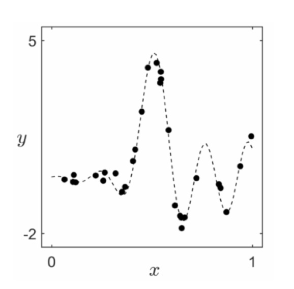
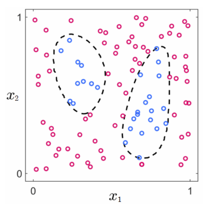
- Pretty hard! And we can visualize these!
- And we have no chance of doing this when we have more than $N = 2$ inputs (we can't visualize!)
- This is where neural networks (as well as kernels and trees) come in!